Speaker Recognition using Python and Machine Learning
Introduction / Project Overview
I had been wanting to learn more about machine learning (as well as Python), and I was really excited to take a “Neural Network and Fuzzy Logic” course my last semester. But unfortunately, it got canceled due to low enrollment. So when I found out that my Fractals class had a final project with a free choice of topic, I took advantage of the opportunity and did mine on machine learning.
For this project, I used the popular machine learning algorithm Gaussian Mixture Models (GMM) to train models to recognize the speakers of some commonly used “command” words. This project was implemented in Python, which I’m still new to, so I followed a base code and modified it to run on Python 3.
Index
Background / Theory
Connection to Fractals
Machine Learning Process
— Dataset Selection
— Pre-processing
— Feature Extraction
— Model Training
— Validation Testing
Results and Discussion
Future Work
Repository
Background / Theory
Speaker Recognition
Speaker recognition: To identify a person based on the characteristics of their voice
This is different from speech recognition, which identifies the words spoken, regardless of speaker.
Speaker recognition can be text-dependent (system can only recognize the speaker when using specific command/trained words) or text-independent (system can recognize the speaker using any words). For example, smart home assistants are text-indepdent — after they learn the user’s voice from a (relatively) small amount of voice data, they’re able to recognize the user, regardless of what they’re saying.
Speaker recognition systems can also be extended to perform speaker verification/authentication. By combining with speech recognition such that the system learns the users’ names, such a system can determine whether the speaker is who they say they are.
Time Domain vs Frequency Domain
Most people are used to seeing voice/sound as a time domain waveform, like this one:
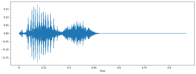
This is the waveform of one of the speakers in the dataset saying the word “yes”, plotted using Librosa in Python. Knowing what word was said, you can kinda see in the wave the structure of the word: “ye-s”. But as we learned in school/engineering classes, time domain representation doesn’t give us a whole lot of useful information to work with. So we use frequency domain instead.
So here’s the same voice clip in the frequency domain, or its spectrogram:
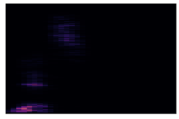
Well it tells us what frequencies are there but… it’s not a lot to work with.
Here’s another spectrogram of another speaker saying the same word:
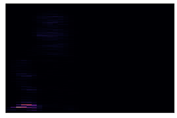
Well you can tell it’s different, but it’s not that different.
How Humans Hear and the Mel Frequency Scale
How are we humans able to differentiate between and recognize all the voices we hear? Well one thing to remember is that we don’t hear differences in frequencies, or pitches, linearly. For example, 100Hz and 200Hz sound farther apart than 1000Hz and 1100Hz, even though both sets have a 100Hz difference between them.
So this is where the Mel frequency scale comes in.
The Mel frequency scale is a nonlinear scale which more closely approximates the human auditory system’s response to different pitches, or frequencies. There isn’t a standardized formula for calculating the Mel frequency equivalent, but here’s a popular one:
\[m = 2595\log_{10}(1\ +\ \frac{f}{700})\]And when plotted against the Hertz scale, it looks like this:
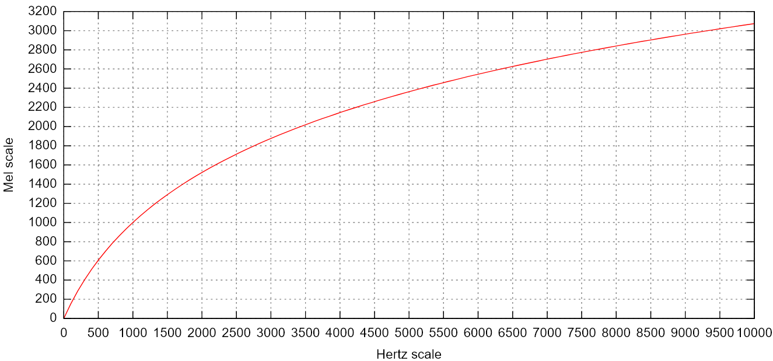
(You can read more about the Mel scale on Wikipedia, which is also where I got the image of the above plot.)
Mel-scaled Spectrogram
From the formula and the plot we can see that humans hear different frequencies logarithmically. So what if we plot our spectrogram using the Mel scale?

Well that’s… better. But it’s still pretty sparce. Are we missing something else? Maybe something that we also hear logarithmically?
Oh! Volume! How could we forget about the decibel scale? So let’s try plotting our Mel-scaled spectrogram with the amplitude scaled in dB.
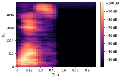
Wow look at that! That’s a lot more information available for us (or a computer) to analyze.
In fact, another popular method for training speaker recognition models is to feed these Mel-/dB-scaled spectrograms into a neural network. Then it simply becomes an image classification problem. It was actually one of the methods that I looked into for this project, but since I wanted to learn about machine learning before trying to get into deep learning, I decided against using it.
(Mel frequency) Cepstrum
Because we’re not using the spectrogram images, we need to use some other way to extract some features to train our models with. One common way in audio signal processing to represent the power spectrum of a sound is by its “cepstrum”. Or more specifically, for audio signals, the Mel frequency cepstrum (MFC).
A cepstrum is basically the “spectrum of a spectrum”. It shows the rate of change/periodicity in the different spectrum bands. For the Mel frequency cepstrum, the power spectrum is mapped to the Mel scale.
Just as we can derive Fourier coefficients for a Fourier series, we can also derive Mel frequency cepstral coefficients (MFCCs) for a MFC. This is commonly done by:
- Taking the Fourier Transform of a signal
- Mapping the power spectrum to Mel scale
- Taking the log of the Mel-scaled power spectrum
- Taking the inverse Fourier Transform of the power spectrum to the "quefrency" domain (time in samples)
- The resulting amplitudes are the cepstral coefficients.
(You can read more about the MFC on Wikipedia)
Although MFCCs give us information about the spectrum of a speech signal, they’re limited to a particular frame. This is similar to the study of motion: A moving particle can be described by its (instantaneous) position, but to know its motion, we need to find its velocity and acceleration, the first and second derivatives of its position. Likewise, speech signals are time-varying, and there’s information in the way the MFCCs change.
In this case, the first and second derivatives are called the differential and acceleration coefficients, or the delta and delta-delta MFCCs.
The delta MFCCs can be found using the following formula:
\[d_t\ =\ \frac{\sum_{n=1}^{N} n(c_{t+n}\ -\ c_{t-n})}{2\sum_{n=1}^{N} n^2}\]where \(d_t\) is the delta coefficient, from frame \(t\) computed in terms of the static coefficients \((c_{t+n}\ -\ c_{t-n})\), and a typical value for \(N\) is 2. The delta-delta coefficients can be calculated similarly by replacing the static coefficients in the formula with the delta coefficients.
Researchers have found that using just the delta coefficients improved the performance of speech (and speaker) recognition systems.
You can read more about them (and about MFCCs as well) here and here.
Gaussian Mixture Models
Gaussian Mixture Models (GMM) is a commonly-used method in unsupervised machine learning. A lot of information, as well as the math behind it, can be found on this blog(, from which I also grabbed some images below). For the purpose of this project, here’s a brief conceptual summary.
Let’s say we’ve extracted the features from our dataset, and plotted on a graph, they look like this:
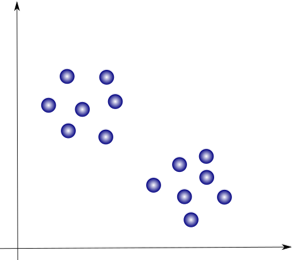
We can see pretty clearly that they can easily be grouped into 2 clusters like this:
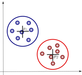
This is the basis behind another popular alagorithm, “K-means clustering”. This method finds the mean, or centroid, of each cluster (μ1 and μ2 in the image) and their distances from each datapoint. The datapoints are grouped into a cluster based on proximity until the results converge. This is known as a hard clustering method, in which each point belongs to only one cluster.
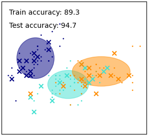
Gaussian Mixture Models (GMMs), on the other hand, is a soft clustering method. Each cluster is represented by a Gaussian, which describes the probability that the data points belong to that cluster.
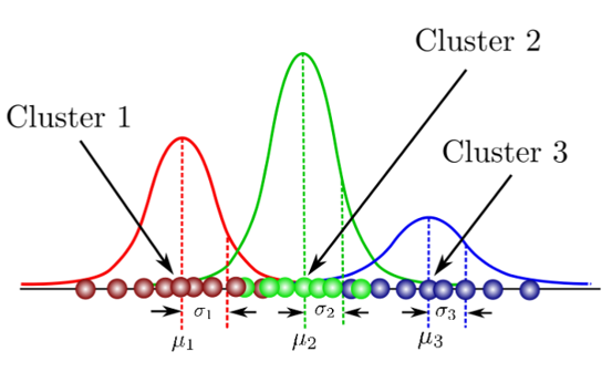
Some important differences to note are that data points can belong to more than 1 cluster, such that cluster boundaries can overlap, and the clusters are not necessarily circular, as illustrated by this image from a SciPy GMM demo.
Connection to Fractals
Scale
One feature of fractals that we discussed in class is “scale”, and the idea that what we can see depends on how closely we “zoom in”.
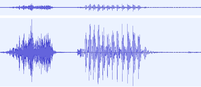
Here are 2 different versions of the same waveform of one of the voice clips used. In the top waveform, most of the end just looks like noise. But if we zoom in closer, we get the bottom waveform, and we can see that there’s actually a little something right at the end there. That’s actually the “p”-sound in the word “stop”, an important feature! If we hadn’t looked closer, we might have dismissed it as noise and accidentally trimmed part of the word.
Self-similarity
The other feature of fractals that people are most familiar with is of course the concept of “self-similarity”. In this case, rather than exact self-similarity, we’re looking instead at stochastic self-similarity. When it comes to speech, even if we try, we can’t say the same word exactly the same twice. But yet, we still recognize the word. We also recognize when different people are saying the same word. The fact that we can train a machine to recognize different speakers as well as words, is based on the premise that there is some stochastic, or statistic, self-similarity that can be recognized.
Here we have 2 instances each of 3 different people saying the word “yes”.
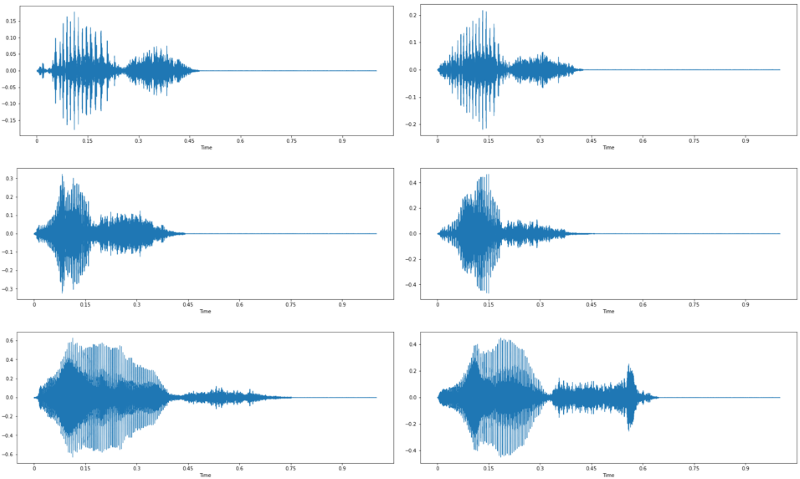
We can see that the waveforms for each speaker definitely look alike. There is also some similarity between all these instances, especially when compared to the waveform of the word “stop” above.
We can also look at the Mel-scaled spectrograms of these waveforms.

In the frequency-domain, the similarities between the 2 instances of each speaker is even more obvious!
Machine Learning Process
Dataset Selection
For this project, I used the “Speech Command Dataset” created by the TensorFlow and Google AIY teams. It contains 65,000 1-second-long utterances of 30 short words submitted by members of the public through the AIY website. These include commonly-used “command” words (yes, no, stop, on, off), digits, directions, as well as some miscellaneous words and names.
My motivation behind using this dataset rather than other popular speech datasets like VoxForge was because of the fact that this project was for a Fractals course. I wanted to have example clips of different people saying the same words multiple times in order to show the self-similarities in the time and frequency domains.
As a first-time project, I decided to use a smaller subset of the dataset. 6 speakers were randomly selected based on the criteria that they had 5 clips for each word, and ended up being 5 male and 1 female. The words chosen were “yes”, “no”, “stop”, “go”, and “up”. During the whole process, between 5-11 clips/speaker were used for training, and 1 clip/speaker was used for testing.
Pre-processing
As the clips were submitted by the public, the quality vary vastly. It also seemed that speakers often recorded clips of the same words consecutively, so there was common background noise in all clips. I wanted to make sure the model was based on the voice and not the background noise as much as possible, so some pre-processing was done before training.
All data were pre-processed manually using Audacity as following:
- Trim word
- Align to start
- Zero-padding for 1-sec clip
Feature Extraction
Using the python_speech_features library, 20 Mel frequency ceptral coefficients and 20 delta Mel frequency cepstral coefficients are extracted for a total of 40 training features.
import numpy as np
from sklearn import preprocessing
import python_speech_features as mfcc

def calculate_delta(array):
  """Calculate and returns the delta of given feature vector matrix"""

  rows,cols = array.shape
  deltas = np.zeros((rows,20))
  N = 2
  for i in range(rows):
    index = []
    j = 1
    while j <= N:
      if i-j < 0:
        first = 0
      else:
        first = i-j
      if i+j > rows-1:
        second = rows-1
      else:
        second = i+j
      index.append((second,first))
      j+=1
    deltas[i] = ( array[index[0][0]]-array[index[0][1]] + (2 * (array[index[1][0]]-array[index[1][1]])) ) / 10
  return deltas

def extract_features(audio,rate):
  """extract 20 dim mfcc features from an audio, performs CMS and combines
  delta to make it 40 dim feature vector"""

  mfcc_feat = mfcc.mfcc(audio,rate, 0.025, 0.01,20,appendEnergy = True)
  mfcc_feat = preprocessing.scale(mfcc_feat)
  delta = calculate_delta(mfcc_feat)
  combined = np.hstack((mfcc_feat,delta))
  return combined
Model Training
Files to be used for training are enrolled in the text file, grouped by speaker. Features (MFCCs and delta-MFCCs) are extracted for each file and concatenated in a vector. When the specified number of files (10/speaker in this case) has been reached, model training is done using the sklearn GMM function. The trained model is then saved in a separate folder to be used for testing.
import pickle as cPickle
import numpy as np
from scipy.io.wavfile import read
from sklearn.mixture import GaussianMixture
from speakerfeatures import extract_features
import warnings
warnings.filterwarnings("ignore")

#path to training data
source   = "training_data\\"

#path where training speakers will be saved
dest = "speaker_models\\"
train_file = "training_set_enroll.txt"
file_paths = open(train_file,'r')

count = 1
# Extracting features for each speaker (11 files per speakers)
features = np.asarray(())
for path in file_paths:
    path = path.strip()
    print(path)

    # read the audio
    sr,audio = read(source + path)

    # extract 40 dimensional MFCC & delta MFCC features
    vector   = extract_features(audio,sr)

    if features.size == 0:
        features = vector
    else:
        features = np.vstack((features, vector))
    # when features of 11 files of speaker are concatenated, then do model training
    if count == 11:
        gmm = GaussianMixture(n_components = 8, max_iter = 200, covariance_type='diag', n_init = 3)
        gmm.fit(features)

        # dumping the trained gaussian model
        picklefile = path.split("-")[0]+".gmm"
        cPickle.dump(gmm,open(dest + picklefile,'wb'))
        print('+ modeling completed for speaker:',picklefile," with data point = ",features.shape)
        features = np.asarray(())
        count = 0
    count = count + 1
Validation Testing
Files to be tested are enrolled in the text file. Each file is compared with the trained models. The most similar is declared the “winner”.
import os
import pickle as cPickle
import numpy as np
from scipy.io.wavfile import read
# from speakerfeatures import extract_features
import warnings
warnings.filterwarnings("ignore")
import time

#path to training data
source   = "test_data\\"
modelpath = "speaker_models\\"
test_file = "test_set_enroll.txt"
file_paths = open(test_file,'r')

gmm_files = [os.path.join(modelpath,fname) for fname in
              os.listdir(modelpath) if fname.endswith('.gmm')]

#Load the Gaussian Speaker Models
models    = [cPickle.load(open(fname,'rb')) for fname in gmm_files]
speakers   = [fname.split("\\")[-1].split(".gmm")[0] for fname
              in gmm_files]

# Read the test directory and get the list of test audio files
for path in file_paths:

    path = path.strip()
    print(path)
    sr,audio = read(source + path)
    vector   = extract_features(audio,sr)

    log_likelihood = np.zeros(len(models))

    for i in range(len(models)):
        gmm    = models[i]  #checking with each model one by one
        scores = np.array(gmm.score(vector))
        log_likelihood[i] = scores.sum()

    winner = np.argmax(log_likelihood)
    print("\tdetected as - ", speakers[winner])
    time.sleep(1.0)
Results and Discussion
Trained models achieved 67-100% accuracy in speaker recognition depending on test data used.
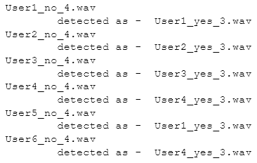
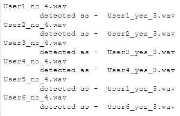
Due to the small dataset used (about 5-13 seconds, including silence, of voice clips per speaker), in general the model is only successful about 4-5 out of 6 times at identifying the speaker. The model tends to be more successful if the test word is one that it has “heard” at least once.
However, when the model is trained on the same word (4x) used for testing, even though the test clip is previously unseen, the model is able to identify the speaker 100% of the time.
It was also accidentally found that the system seemed able to recognize between different words, implying that the system could be used to perform speech recognition instead/as well.
Future Work
To improve performance, more voice samples (available in the main Speech Commands Dataset) will likely be needed for training. Data can also be augmented (for example by introducing noise) in order to increases the robustness of the model.
Other ML/DL algorithms could be implemented instead/in addition to GMM.
It should also be possible to extend this model to perform speech recognition and/or speaker verification.
Repository
The full code can be found in the repository here.